Computer Vision
Motion Approximation From Optical Flow
About the Project
The use of computer vision has skyrocketed over the past few decades, especially for motion analysis. For this project, I demonstrated the use of vision processing techniques to estimate the state of a mobile robot. Achieving robust, real-time performance is computationally intensive, so the algorithms explored were selected primarily for their efficiency. The Shi-Tomasi improved corner detection algorithm was coupled with the Lucas-Kanade optical flow algorithm, and the output was then combined with data from an Inertial Measurement Unit (IMU) via an Extended Kalman Filter (EKF) to estimate robot motion.
Skills Involved
- OpenCV
- Vision Processing in C++
- Optical flow
- Motion tracking
- Camera calibration
- Visual odometry methods
- Camera stabilization techniques
- Structure from motion
- 3D reconstruction from stereo
Procedure
Two different computer vision methods were tried and their results compared. Both methods first estimate the camera motion from optical flow data and use the rigid transform between camera and robot chassis to then estimate robot motion. In method 1, the Essential Matrix was decomposed to a transformation matrix (which consists of a rotation and translation). For method 2, a simpler projective transform was used, since the transform between camera and ground frames was known. A projective transform is computationally cheap, requiring only a single matrix multiplication operation for each tracked point.
The first technique, unfortunately, did not work very well. The Essential Matrix calculation often returned invalid results, and the decomposition process produces 4 unique solutions, so even valid results had to be sifted through to find the correct one. There are many reasons for the invalid returns, including:
- Too little camera motion from frame-to-frame
- Noisy image data (especially when moving)
- Singular planar surfaces (such as floors) are a degenerate case
- Scale ambiguity of the method
Needless to say, this method was not ideal. Furthermore, it's much more computationally expensive than the 2nd method. Meanwhile, the projective transform worked surprisingly well. It had somewhat large error at high speeds, but that could be overlooked for the purposes of this project.
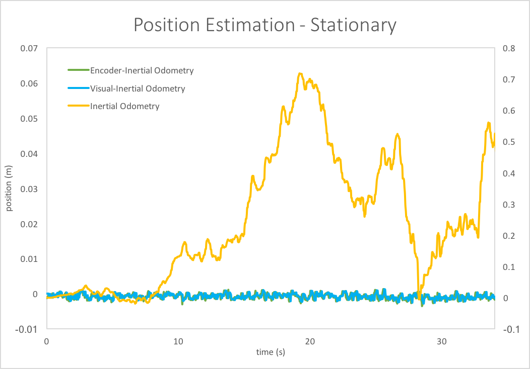
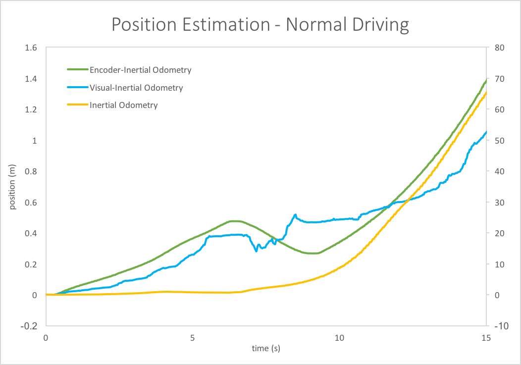
After collecting test data and comparing the 2 methods, it was clear that the projective transform was the best method both from an efficiency and accuracy standpoint. The resulting visual odometry was also far more accurate than inertial navigation alone (i.e. using only the IMU to estimate state).
The results of both are shown in the adjacent plots, as well as data for wheel encoder odometry. In the Stationary test, both visual and encoder odometry accumulate almost zero positional change over 35 seconds (as expected). Inertial navigation, however, drifts almost 75 cm and back in that same time frame. A similar result is obtained for the Normal Driving test - the visual and encoder odometry graphs give relatively consistent predictions, while the IMU graph dwarfs them both in scale (note there are 2 separate axes - one for encoder & visual, the other for inertial - which vary by a factor of nearly 50).
Learn More
This was my final project for EECS 423: Advanced Computer Vision at Northwestern. Download the software package from GitHub to try it for yourself. The README should contain all necessary information to get it running.